No products in the cart.


18 min read
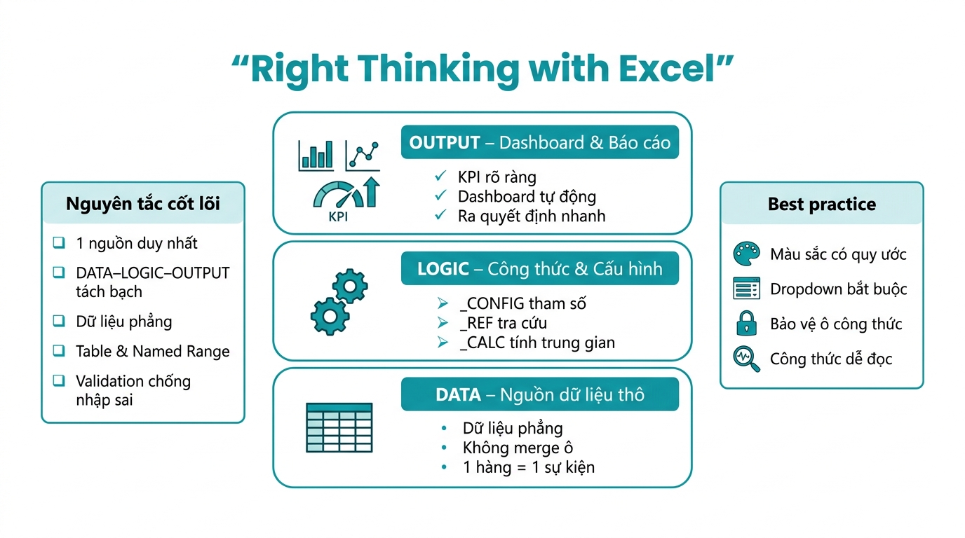
Short answer: Properly designing an Excel file means separating it into three non-mixing layers — DATA INPUT (where data is entered), LOGIC LOGIC (where data is processed), OUTPUT OUTPUT (where results are read) — along with the principle of a single source of truth for all changeable parameters. Most cluttered Excel files aren’t due to weak formulas but because these three layers are mixed into one sheet, leading to a situation where, after a few months, no one — including the file creator — understands it anymore.
Many people learn Excel by searching for formulas for specific problems. VLOOKUP, SUMIF, IF nested in IF — they learn these but still create cluttered files, spend hours finding errors, and are afraid to let others use them because they fear the file will be “broken”. The problem isn’t Excel. The problem is that formulas are just tools, and what they haven’t learned is design designing the file before starting work
Compare two people who learn Excel for three months. Person A opens Excel and starts entering data immediately, thinking on the fly, adding new columns as needed, coloring for aesthetics, and copying formulas from Google. Person B spends fifteen minutes sketching on paper: what the input data is, what reports are needed, who will use the file, how many sheets, and what each sheet does — before opening Excel. After three months, Person A’s file is incomprehensible, even to themselves. Person B’s file still runs smoothly, can be expanded, and a new user can learn it in thirty minutes. The difference lies entirely in systems thinking.
Designing an Excel file is like designing a house. You can’t build walls before having a blueprint. You can’t cram bedrooms, kitchens, and living rooms into one room. Each area must have a clear function and not overlap. Electrical and water lines must be routed correctly — not running wildly through walls.
Core principle: Data enters one place. Logic is processed in one place. Results are displayed in one place. These three layers never mix.
Article contents
This is the foundation of everything. Any Excel file — whether simple or complex — should be built on these three layers. When these layers are mixed, no formula is smart enough to save the file from becoming disorganized after six months.
DATA is where you enter raw data. No flashy colors, no complex formulas, no merged cells. Just clean, consistent, raw data. The right mindset: your DATA sheet is your data foundation — it doesn't need to be visually appealing, it needs to be accurate and consistent.
Practical example for an F&B store managing sales:
| Ngày | Product code | Dish name | Quantity | Unit | Selling price | Sales channel |
|---|---|---|---|---|---|---|
| 01/04/2025 | PHO-01 | Rare beef noodle soup | 50 | tô | 65,000 | At the restaurant |
| 01/04/2025 | BUN-02 | Hue beef noodle soup | 30 | tô | 55,000 | GrabFood |
| 01/04/2025 | PHO-01 | Rare beef noodle soup | 12 | tô | 65,000 | ShopeeFood |
| 02/04/2025 | COM-05 | Broken rice with grilled pork | 45 | phần | 45,000 | At the restaurant |
Seven golden principles for the DATA sheet, applicable to all types of files without exception:
Common errors to avoid: adding a secondary header row like “=== April ===” between data to separate by month is structurally incorrect — instead, add a “Month” or “Quarter” column and use filters/groups to separate. Merging cells like “Beef Pho” for three identical orders is also structurally incorrect — repeat “Beef Pho” in each row; flat data with each row independent is a requirement for Pivot Tables to work.
LOGIC is the “factory” of the file — where all processing takes place. End-users typically don't need to look at this. Sheets in this layer are often hidden or named with special characters to distinguish them. Three standard sheet types in the LOGIC layer:
Sheet _CONFIG — system configuration and parameters. Contains all fixed numbers: exchange rates, tax rates, service fees, catalog lists (products, employees, sales channels), warning thresholds (minimum inventory, sales targets), and company information (name, address, tax code) for reporting. Rule: any number that can change over time — must be in _CONFIG, never hard-code into formulas.
Sheet _CALC — intermediate calculation tables. Contains complex calculations that don't need to be displayed directly: cost calculations based on recipes (for F&B), cost allocation tables by period, and SUMIF/SUMPRODUCT aggregations from previous DATA before being displayed on the dashboard. For example, F&B: _CALC Contains recipe tables with ingredient ratios and calculates the cost of each dish; the dashboard simply references the results from here.
Sheet _REF — reference tables and catalogs. Contains lookup tables: product code tables with full category names and selling prices, employee tables with departments and positions, province tables with economic regions and shipping fees. When there are tables _REF standard, all VLOOKUP/XLOOKUP formulas reference this sheet — never the DATA sheet.
Sheet naming convention in the LOGIC layer: starts with an underscore to automatically group and easily recognize, or uses lowercase (config, calc, ref) distinguish from uppercase for OUTPUT and DATA. Shade the LOGIC tab sheet gray to differentiate it from DATA (white) and OUTPUT (blue).
OUTPUT is where users look to make decisions. Information is filtered, summarized, and visualized. No cells are manually entered here — all are formulas referencing LOGIC or DATA. Five principles for good OUTPUT design: place the most important information in the top-left corner (people read from left to right, top to bottom); group related information together, avoiding scattered data; use color and icons purposefully, not for decoration; each figure must have context (revenue of 50 million is meaningless without comparison); avoid too many numbers, selecting 5-7 key KPIs instead of dumping all data.
Monthly Dashboard for an F&B establishment — what needs to be displayed:
| KPI | This month | Previous month | Target | Status |
|---|---|---|---|---|
| Revenue | 52,400,000 | 48,200,000 | 50,000,000 | 🟢 +8.7% vs target |
| Cost of goods sold (COGS) | 21,800,000 | 19,500,000 | ≤ 22,000,000 | 🟢 41.6% — stable |
| Gross profit | 30,600,000 | 28,700,000 | 28,000,000 | 🟢 +6.6% |
| Number of transactions | 1,240 | 1,180 | 1,200 | 🟢 Exceeding target |
| Inventory below threshold | 3 items | 1 item | 0 | 🔴 Needs additional input |
The “Status” column is created using Conditional Formatting combined with IF formulas — fully automated, no manual input. The owner opens the file in the morning and can see what needs to be done in just three seconds by looking at the dashboard.
This is the most important principle and also the most frequently violated one. A typical error seen in most SME files: the cost of a dish is manually entered in the inventory sheet, entered again in the sales sheet, and entered once more in the monthly report sheet. Three months later, the three places have three different numbers — and no one knows which one is correct.
Or more commonly: the 8% VAT rate is hardcoded into 47 different formula cells. When the government changes the tax rate, the file owner has to search for and update each cell individually — and will likely miss a few places.
The correct ruleany information that may need to be changed or used in multiple places — must have a single original cell in the _CONFIGAll other places can only reference that cell using a formula.
A real-life example for exchange rates and tax rates:
Sheet _CONFIG:
B2 = 25,400        ← USD/VND exchange rate — ONLY UPDATE HERE
B3 = 8%            ← VAT — ONLY UPDATE HERE
B4 = 3.5%          ← GrabFood fee — ONLY UPDATE HERE
B5 = 2.2%          ← ShopeeFood fee — ONLY UPDATE HERE

Sales sheet (formula):
= C5 * _CONFIG!$B$2          ← Convert USD to VND
= D5 * (1 + _CONFIG!$B$3)    ← Add VAT
= E5 * (1 - _CONFIG!$B$4)    ← Subtract Grab fee
When Grab increases its fee from 3.5% to 4% — you only need to update one cell (_CONFIG!B4), the entire file updates in a few seconds.
This principle also applies to product categories. Instead of entering product names directly into each row in the DATA sheet, create a category table in _REF — the DATA sheet only enters the product code, while the name, price, and category are all looked up from the REF table. When the selling price changes, you only need to update one cell in _REFthe entire sales history remains correct (since sales are taken from the entered unit price column), but the new price analysis reports update automatically.
Single Source of Truth is the principle that each piece of data should be stored in only one place. Everywhere else that needs that data should reference it, not copy the value.
This concept is often unknown to self-taught Excel users — and it makes a huge difference between an analyzable file and one that's just for viewing. Excel is designed to work with tabular data. All of Excel's powerful tools — SUMIF, COUNTIFS, Pivot Table, charts, Power Query — work best with flat data.
The wrong approach — data in wide formatMany people create employee sales reports in this way:
| Employee | January | February | March | April | May | June |
|---|---|---|---|---|---|---|
| Nguyễn An | 45M | 52M | 48M | 61M | 55M | 58M |
| Trần Bình | 38M | 41M | 44M | 39M | 47M | 52M |
| Lê Châu | 29M | 33M | 31M | 35M | 42M | 38M |
This method looks “compact” but is extremely limited. Want to calculate the total Q1 sales for the entire team? You have to do it manually. Want to filter to see which month has an employee with sales under 40M? Can't do it. Adding a new month? You have to add a column, and all aggregate formulas need to be revised. Pivot Table? Almost impossible to use.
The correct way — flat data (long/flat format):
| Employee | Month | Năm | Sales | Vùng |
|---|---|---|---|---|
| Nguyễn An | 1 | 2025 | 45,000,000 | Southern region |
| Nguyễn An | 2 | 2025 | 52,000,000 | Southern region |
| Trần Bình | 1 | 2025 | 38,000,000 | Northern region |
| Trần Bình | 2 | 2025 | 41,000,000 | Northern region |
Now you can do it all:
' Total Q1 sales for the entire team:
=SUMPRODUCT((DOANH_SO[Year]=2025)*(DOANH_SO[Month]<=3)*DOANH_SO[Sales])

' Average monthly sales of Nguyễn An:
=AVERAGEIF(DOANH_SO[Employee],"Nguyễn An",DOANH_SO[Sales])

' Pivot Table: drag and drop for 30 seconds to get a report by region × month
And most importantly: adding new monthly data is just adding a row, without modifying any formulas.
Summary: Data in “long” format is always easier to analyze than data in “wide” format. If your file is in a wide format, that's a clear sign that Pivot Table and automatic reports will never work.
Many Excel users, even after a decade, have never used Excel Table (Ctrl+T). This is one of the most powerful and least known features — a must-have for a sustainable file.
Excel Table automatically does what you're doing manually: automatically expands the data range when adding new rows (SUMIF formula doesn't need to update the range); column names replace cell addresses in formulas (=[@Doanh_so] * [@Gia_von] easier to read =D2*E2); automatic filter is added to the header; alternating format (banded rows) makes it easier to read and is automatically applied to new rows; total row (Total Row) with dropdown selection of SUM, AVERAGE, COUNT, MAX, MIN.
How to create: click on any cell in the data range → Ctrl+T → OK. Then, rename the Table instead of “Table1”: select the tab Table Design; enter the name in the box Table Name (for example SALES, INVENTORY, EMPLOYEE).
After naming, the formula becomes self-explanatory:
Instead of:
=SUMIF($A$2:$A$1000, "Grab", $D$2:$D$1000)

Write as:
=SUMIF(SALES[Sales Channel], "Grab", SALES[Sales])
The second formula is easy to understand for anyone: calculate the total Sales from the table SALESfilter by Sales Channel using “Grab”. No need to open another sheet to decode cell addresses.
In addition to Excel Table, you should combine Named Ranges for important cells or reference ranges. When to use Named Ranges instead of (or in combination with) Excel Table? For single cells like exchange rates, tax rates, warning thresholds; for fixed ranges like category tables, price tables; when you need to reference cross-sheet easily.
Naming Method: select a cell or range → click on the Name Box (cell address display, top left corner) → type a name → Enter. Or use Formulas → Name Manager for centralized management.
Good naming convention:
| Loại | Example Name | Meaning |
|---|---|---|
| Single Parameter | USD Exchange Rate, VAT, TARGET_LIST | Single Cell _CONFIG |
| List | Product List, DS_KENH, DS_NHAN_VIEN | Dropdown validation area |
| Reference table | BANG_GIA, BANG_GIA_VON, BANG_CUOC_VAN | VLOOKUP/XLOOKUP area |
Actual results when combining Excel Tables with Named Ranges:
Instead of:
=VLOOKUP(A2, _REF!$A$2:$F$200, 5, 0) * Sheet3!$B$2

Write:
=XLOOKUP([@Ma_SP], BANG_GIA[Ma_SP], BANG_GIA[Gia_ban]) * TY_GIA_USD
When updating exchange rates or price lists, make changes in the right place without altering formulas.
Colors in Excel are not just for aesthetics. Colors are a visual language that conveys information about the structure and status of a file. Standard color system — applied consistently across all files:
| Background color | Meaning | Cell type | User capabilities |
|---|---|---|---|
| Light yellow (#FFF2CC) | Data entry | Input cell | Freely editable |
| Light blue (#DEEAF1) | Auto formula | Formula cell | Not manually editable |
| ↵ White / very light gray | Raw data | Data cell | Enter according to regulations |
| 🟫 Dark gray + white text | Header | Column header | Do not edit |
| 🟢 Light green (#E2EFDA) | Good result / meets target | Conditional | Automatic based on logic |
| 🔴 Light red (#F8CBAD) | Warning / below threshold | Conditional | Automatic based on logic |
| 🟠 Light orange (#FCE4D6) | Near threshold / needs attention | Conditional | Automatic based on logic |
The first golden rule: anyone looking at your file for the first time should immediately understand which cells are input and which are results — just by color, without explanation. The second golden rule: sheet tabs should also be colored — white or default for DATA, gray for LOGIC (_CONFIG, _CALC, _REF), green for OUTPUT/Dashboard, red for temporary or pending sheets.
Practical Conditional Formatting — inventory example:
Column G = Current inventory
Column H = Minimum inventory level (from _CONFIG)

Rule 1: If G < H       → red background + bold red text ("Need to order")
Rule 2: If G < H*1.2   → orange background ("Running low")
Rule 3: If G >= H*2    → green background ("In stock")
No need to look at the numbers, just look at the color to know what to do.
The best Excel file is one that cannot be entered incorrectly — or if entered incorrectly, it warns immediately. Core principle: design for failureAssuming the user sẽ Incorrect input, and designing to prevent it from the start. Four types of validation you should know:
In a real-world order management file, the name "Grab Food" had seven different spellings in the same column: "Grab", "GrabFood", "grab food", "GRAB", "Grab Food", "grab", "GrabFoods". Result: sales channel reports were completely incorrect. A dropdown list solves this problem in two minutes.
Step 1: Create a list in _REF (e.g., DS_KENH_BAN)
    In-store
    GrabFood
    ShopeeFood
    BeFood
    Baemin

Step 2: Select the sales channel column in the DATA sheet
Step 3: Data → Data Validation → Allow: List
Step 4: Source: =DS_KENH_BAN
Step 5: Error Alert → "Invalid sales channel. Please select from the list."
Users can only select from the dropdown — cannot enter incorrectly. Advanced tip: dependent dropdown (dependent dropdown) — select a category and the product dropdown only shows products belonging to that category; use the INDIRECT Combine Named Ranges with category-based naming.
Quantity column: Allow = Whole number, Minimum = 1
Selling price column:  Allow = Decimal, Minimum = 0
Date column: Allow = Date, limited from the opening date to todayEnsure the product code always starts with uppercase letters:
=AND(LEN(A2)=6, EXACT(LEFT(A2,3), UPPER(LEFT(A2,3))))Prevent duplicate entries in the employee code column:
=COUNTIF($A$2:$A$1000, A2) = 1After designing, lock the entire sheet and only allow input in designated cells:
Step 1: Ctrl+A → Format Cells → Protection → uncheck "Locked"
Step 2: Select INPUT cells only → recheck "Locked"
         (Reverse logic: default is unlocked, only lock cells that need protection)
Step 3: Review → Protect Sheet → set a password
Result: users can only click on the yellow cell (INPUT). All formula cells are automatically protected and cannot be broken, even accidentally.
A good formula is not only accurate — it must be easy to read, verify, and modify. Three techniques completely change the quality of a formula:
IFS instead of nested IFsFour-level nested IF is nearly impossible to verify visually:
❌ Hard to read (4-level nested IF):
=IF(D2>50000000,"Excellent",IF(D2>40000000,"Good",IF(D2>30000000,"Fair",IF(D2>20000000,"Needs improvement","Fail"))))

✅ Easier to read with IFS (Excel 2019+):
=IFS(
    D2 > 50000000, "Excellent",
    D2 > 40000000, "Good",
    D2 > 30000000, "Fair",
    D2 > 20000000, "Needs improvement",
    TRUE,          "Fail"
)
Replace VLOOKUP with XLOOKUPVLOOKUP has clear limitations and is very prone to errors when adding columns to the table:
VLOOKUP — limited and error-prone:
=VLOOKUP(A2, BANG_GIA, 4, 0)
                      ↑ What is column 4? Must count manually. Adding a column in between → the number 4 is incorrect.

XLOOKUP — explicit and flexible:
=XLOOKUP(A2, BANG_GIA[Ma_SP], BANG_GIA[Gia_ban], "Not found")
           ↑ Where to find A2?  ↑ return which column?     ↑ what to return if not found?
Break down complex formulasInstead of writing a 200-character formula, calculate each step in auxiliary columns (which can be hidden later):
Column H (hidden) = Gross Revenue: =[@SL] * [@Gia_ban]
Column I (hidden) = Platform Fee: =[@DT_tho] * XLOOKUP([@Kenh], BANG_PHI[Kenh], BANG_PHI[Phi])
Column J (hidden) = VAT: =[@DT_tho] * THUE_VAT
Column K = Net Revenue: =[@DT_tho] - [@Phi_platform] - [@Thue_VAT]
Now, each step can be checked separately — 10 times easier to debug than a monolithic formula.
I once received two files from two restaurant owners of the same scale and type, with annual revenues of around 2 billion. However, their management files represented two different worlds.
File A — the "emotional file"A single sheet with 47 columns, hundreds of merged cells, and random color fills. Formulas are copied from Google, with half of them returning #REF when adding new rows. Cost is entered manually in three places — with three different numbers. The owner spends two hours per week updating and is still unsure if the data is correct. When new employees join, the owner must spend hours explaining and still monitors them for fear of "breaking the file".
File B — the "design file"Five sheets: DATA, _CONFIG, _CALC, _REFthe Dashboard. Consistent color scheme — yellow for input, green for formulas. All categories are dropdowns from _REFCost and other parameters are centralized in _CONFIGThe dashboard updates automatically when new rows are added to the DATA sheet. The owner spends 15 minutes per week, the data is always accurate, and new employees can use it after 30 minutes without guidance.
File B is not more complex than File A in terms of Excel skills — in fact, it has fewer formulas. The difference lies entirely in the design thinking before opening Excel.
Spending 15 minutes sketching on paper can save dozens of hours of troubleshooting later. Before pressing Ctrl+N, answer these 15 questions on paper, not in your head, divided into three phases:
Problem definition phase:
Data design phase:
Construction phase:
_CONFIG for all adjustable parameters_REF for all categories and lookup tablesIf the fifteen-minute test fails, go back and redesign. Don’t build on a weak foundation.
Excel isn’t difficult. The difficulty lies in systems thinking before opening the file. Everything in this article boils down to one philosophy: design first, build later, never do it the other way around.
A good Excel file isn’t the one with the most formulas, nor the one that looks the prettiest. A good Excel file is one that anyone on the team can understand and use after reading a short guide; data is always consistent, with no conflicting numbers; it’s easy to maintain after six months, even if you don’t remember what you did; it’s difficult to enter incorrect data, thanks to validation and color-coded guidance; and it automatically updates when new data is added.
Next time before pressing Ctrl+N, take a piece of paper and sketch out: what does your DATA sheet contain? Sheet _CONFIG What parameters are needed? What KPIs should the dashboard display? Fifteen minutes sketching on paper will save you dozens of hours of debugging later. When you can answer those questions before opening Excel — you’re on the right track.
✍ Key Takeaways
PRACTICAL TOOLS
Excel File for F&B Quantity and Cost Management — 3-layer standard
The sample file is built on the correct DATA – LOGIC – OUTPUT architecture described in the article. _CONFIG focuses on material costs and parameters, _REF contains recipes for each dish, and the Dashboard automatically calculates gross profit for each dish when you add new orders to the DATA sheet. Validation and Protect Sheet are fully implemented, with a systematic color scheme. It's ready to use and can be expanded as your restaurant grows.
For a medium-sized SME operations management file, designing on paper takes 15-30 minutes, while building the three-layer framework takes 2-3 hours. A file created directly may seem faster initially but accumulates technical debt quickly — after three months, the weekly maintenance time for a poorly designed file can be 5-8 times that of a well-designed one.
No. The three-layer principle and Single Source of Truth work even if you only know SUM, IF, and VLOOKUP/XLOOKUP. More complex formulas can be added as needed. Conversely, learning all formulas without understanding design only creates complex but disorganized files — a common outcome of technically focused Excel courses.
Excel is sufficient for most small businesses with under 50 employees, less than 10,000 data rows per month, and rapidly changing processes. When data exceeds 50,000 rows, requires multiple users to edit simultaneously, or needs a detailed audit trail — that's when you should consider specialized software. Even when switching to software, the three-layer design principle still applies to supplementary Excel reports.
The area with a filter is still a static area — formulas referencing cell addresses ($A$2:$A$1000) and does not automatically expand when adding rows. Excel Table is a dynamic structure — with an automatically expanding range and formulas using column names ([@Sales]), renaming tables to replace sheet names, and any Pivot Table referencing the table will automatically update when refreshed without needing to reconfigure the source.
If the file has fewer than 5,000 rows and fewer than 10 sheets, rewriting it from scratch using a 3-layer architecture is often faster than gradual revisions — taking 1-2 focused working sessions. For larger files, a safe strategy is: keeping the old file running in parallel, building a new one, copying raw data to the new file’s DATA sheet, and verifying that the Dashboard matches the old report for a month before switching completely.
Idea: the “Category” column is selected first, and the “Product” column only shows products belonging to that category. How to do it: in _REF, create Named Ranges with names matching each category (e.g. PHO containing a list of pho dishes, BUN containing a list of noodle dishes). In the Product column, use Data Validation with the source as =INDIRECT([@Danh_muc]) — Excel will automatically look up the Named Range matching the value in the Category column of that row.
Two reasons. First, when tax rates change (as happened when VAT was temporarily reduced by 2% in 2022-2024), you have to find and modify dozens of places — you'll likely miss some. Second, when reading the formula again after six months, the number “0.08” in the formula won't tell you it's VAT or another rate — causing confusion when modifying. Put it into _CONFIG!THUE_VAT You can fix it in one place and immediately understand the meaning of the formula.
Reference: Separation of Concerns principle (Edsger Dijkstra, 1974) applied to spreadsheet design · Single Source of Truth principle in data architecture · Excel Table feature (Microsoft, since Excel 2007) · “Right Thinking with Excel” documentation — BEUP internal framework.
Book a free consultation to explore how BEUP can transform your workflow.
Book a Consultation →Digital Asset Ecosystem & Operating System for individuals & teams.